Smart Antennas and Beamforming, Understanding with GNU : Part 2

Smart Antennas and Beamforming, Understanding with GNU : Part 2  Recap from Part-1 of This Article.

1. There are four types of antenna field regions. Out of those four regions, we discussed radiation pattern of far-field region of an antenna. Also, we plotted a 3D radiation pattern of an antenna with a given radiation intensity.
2. If we have a single antenna then It would require a very tall antenna to direct the radiation towards a specific user. This is the simplest scheme of directing a beam towards a specific user but because of obvious reasons, this scheme is impractical.
3. Antenna array has two or number of antenna elements or antennas. So, the output of an antenna array is equal to the weighted sum of outputs from its elements.  And, if we take multiple antenna elements, arrange them in a specific way then by introducing time delay (we assumed that time-delay is similar to phase-shift) among signal that is coming out of each antenna element would result in a change in direction of the radiation or beam.  This scheme is known as a phased array antenna system.
4. If we increase the number of antenna elements in an array, the output beam from the antenna becomes narrower. And, introducing time delay changes the direction of the output beam.
5. If you noticed octave scripts in part-1 of this article, I used to phase shift instead of time delay. We can easily convert time delay experienced by signal into a phase shift at a given frequency. Consider a linear antenna array system as depicted in Figure 1.  If any signal arrives at degree off at antenna boresight (the axis of maximum gain of a directional antenna.). Then, the time delay can be given by

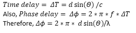
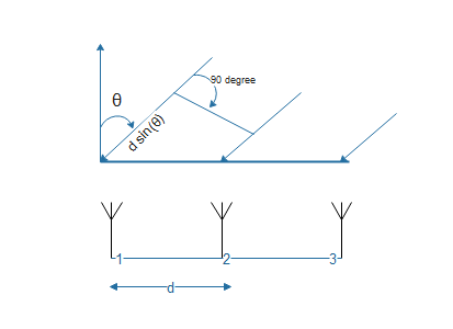
Figure 1: Linear antenna array with three antenna elements, a signal arriving at angle θ

Question to Think About:

• What will happen if we vary the distance between antenna array elements? How will antenna radiation pattern be impacted?
• What will happen if Antenna elements are not arranged in a linear fashion? How about a circular geometry

Smart Antenna System

Let’s define smart antenna system first in our words.

“Smart Antenna system consists of two major blocks. Firstly, an adaptive antenna array block and secondly, a sophisticated signal processing block. These two blocks improve the communication between transmitter and receiver by continuously adapting feedback to antenna array block. Consequently, radiation pattern (Beam) is optimized dynamically according to communication channel characteristics.”

Here, optimized beam pattern means optimizing its direction, shape, and range according to the communication channel.

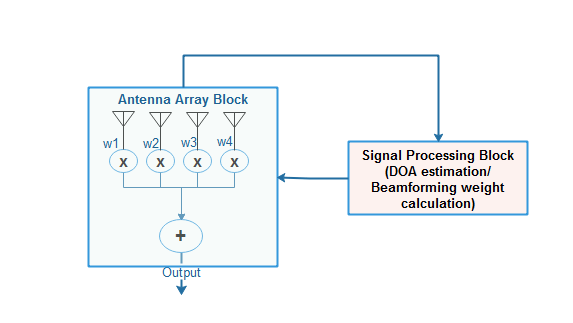
Figure 2: Simplest possible Smart Antenna system, w1, w2, w3, w4 are beamforming weights

The direction of Arrival or Angle of Arrival Estimation Techniques

As it can be seen from figure 2, smart antenna systems use a specific signal property called “Direction of Arrival”, here on referred as DOA, to calculate and update beamforming weights (w1, w2, w3, w4 and so on). So, the main goal here is to find or at least estimate DOA.

It is worth mentioning here that our aim is to calculate beamforming weights and there are many methods other than DOA estimation by which beamforming weights can be calculated. However, we will only focus here on DOA estimation and its use in beamforming weights calculation. Also, we will limit our discussion to uniform linear array (ULA) system, something that is represented in figure-1.

Now, it is to further note that there are many ways by which DOA can be estimated. Below given are some common DOA estimation techniques.

1. Root- MuSIC – Root Multi SIgnal Classification
2. ESPRIT – Estimation of Signal Parameters via Rotational Invariance
3. IQML – Ative quadratic maximum likelihood
4. Root-WSF – Weighted subspace fitting

All the above techniques can be characterized based on coherency, consistency and spectral efficiency.  As shown in below table:

Method	Consistency	Coherent signals	Statistical Performance	Computations
Root-MuSIC	Yes	Yes	Good	Eigenvalue Decomposition, Polynomial
ESPRIT	Yes	Yes	Good	Eigenvalue Decomposition
IQML	Yes	Yes	Good	Iterative
Root-WSF	Yes	Yes	Efficient	Eigenvalue Decomposition, Least Square

In this article, we will focus on a Root-MuSIC method of DOA estimation. But before discussing details of this method, It is important to review mathematics behind these methods in general.

Mathematics of Direction of Arrival or Angle of Arrival Estimation

• Eigenvalues and Eigen Vectors

Many DOA estimation algorithms work on the properties of eigenvalue decomposition. So, this concept is very important to understand.

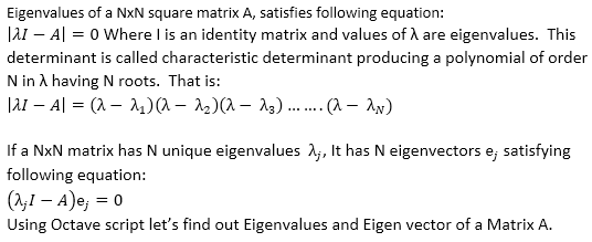
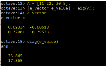
In this example, the first column of e_vector is the first eigenvector and its corresponding eigenvalue is 33.865. Similarly, the second column of e_vector is second eigen vector and its corresponding eigenvalue is -17.865

I would highly recommend a lecture by Professor Gilbert Strang from MIT to understand the concept of Eigenvalues and Eigenvectors below.

• Array Correlation Matrix

Suppose there is an M-element antenna array and D-signals are arriving at it from Θ directions. As shown in the figure below:

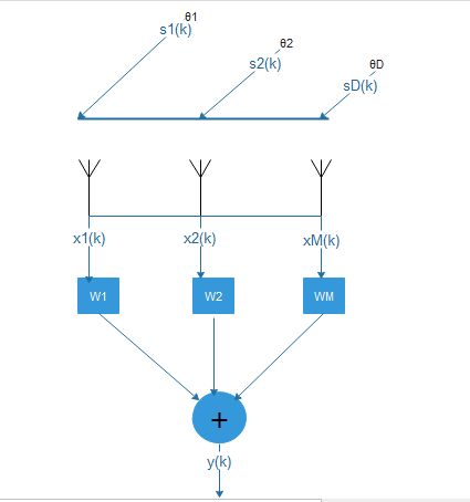
Figure 4: M-element antenna array with D-arriving Signals

 

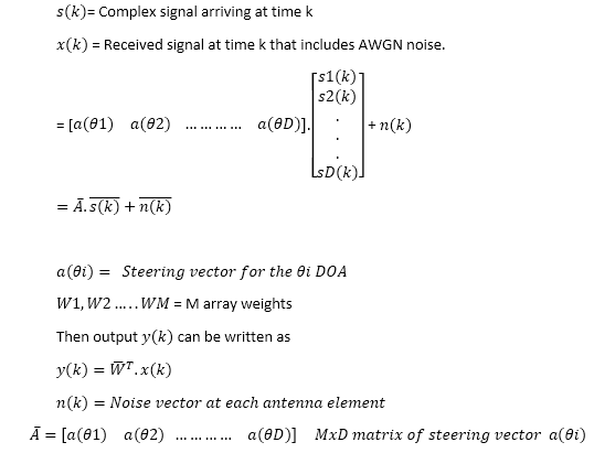
Assuming that all the signals are zero mean, stationary processes then MxM Correlation matrix is composed of signal and noise samples at time k. And, it can be defined as follows:

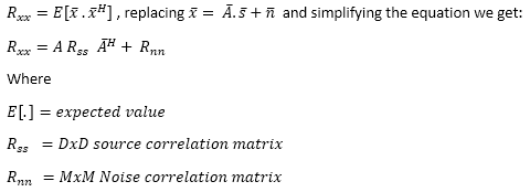
Correlation matrix has M eigenvalues and associated M eigenvectors.  The largest eigenvalues correspond to the signals, while the rest are associated with the noise. So, this correlation matrix can be divided into two subspaces: signal subspace and noise sub-space. Mx(M-D) noise subspace and MDX signal subspace.

In that case (M-D) eigenvectors are corresponding to noise and D eigenvectors are corresponding to the signal.  In other words, D uncorrelated signals incident on an M element array (M > D) produces D signal eigenvalues and M – D noise eigenvalues.

The signal eigenvectors associated with the correlation matrix are the array weights that have beams in the directions of the signals. The noise eigenvectors associated with the correlation matrix are the array weights that have nulls in the directions of the signals.

It is to note that if signals are not zero-mean, stationary processes then correlation matrix is also known as a covariance matrix. So, the heart of the DOA estimation is eigenanalysis of the covariance matrix. Let’s understand eigenanalysis of Covariance matrix further by using Octave.

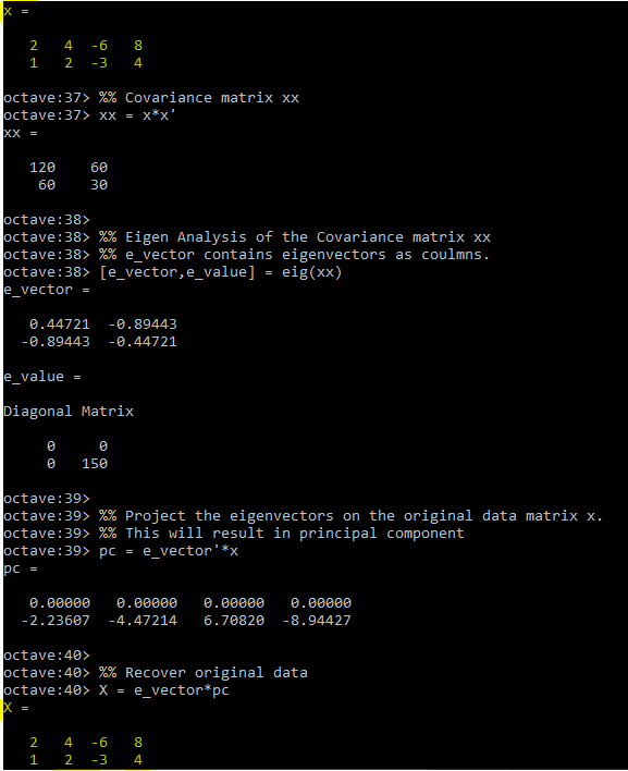
It can be seen above that by doing eigenanalysis of Covariance matrix we are able to recover original data. This is very useful and main building block of DOA estimation algorithms.

Smart Antennas and Beam-forming, Understanding with GNU: Part 3

nown as adaptive antenna array systems are composed of two major blocks; An adaptive antenna array block and a Signal processing block. Signal processing block is responsible for finding and adapting array beamforming weights and antenna array block uses those weights to give final system output. This output is nothing but a narrow beam directed towards a specific user and nulls are directed toward interfering users.

Performance of Antenna array block depends on following:

1. The geometry of the antenna array. Arbitrary array geometry or linear array geometry.
2. Number of antenna array elements
3. Spacing among antenna array elements. Uniformly spaced or arbitrarily spaced.
4. The phase difference between elements.

• Performance of signal processing block depends on the following:

1. Type of algorithm used for estimating weights. For example, the direction of arrival estimates or any other LMS, RMS based method.
2. Further, Direction of arrival estimates also depends on what kind of algorithm is chosen. For example Root-MUSIC, ESPRIT, MVDR (minimum variance distortionless response) etc.

Smart antenna system’s performance depends on the performance of both the constituent blocks.

• The task of finding array beamforming weights is the crux of the system and We limited our discussion to Root-MUSIC DOA estimation algorithm. We described mathematics behind this. In particular, we discussed the correlation matrix which is a special case of the covariance matrix and eigenanalysis of these matrices.
• We saw that correlation matrix consists of two orthogonal subspaces, noise subspace, and signal plus noise subspace. Eigenvalue decomposition, here on EVD, is a way to decompose correlation matrix into these two subspaces. We also saw an example of how EVD can be used for decomposing.
• One other important parameter that was not explicitly mentioned in previous parts of this article but It was buried under Octave script. This Parameter is called Antenna Array factor.

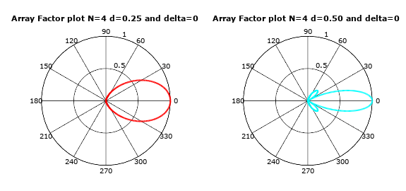
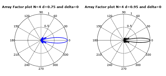
Let’s draw array factor plot for a simple uniform linear array with multiple distances using below octave script.

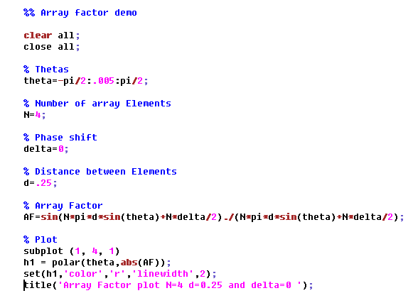
As can be seen from below output plots, the distance between antenna array elements is one major parameter for designing a beamforming array system. As this distance defines beam width.

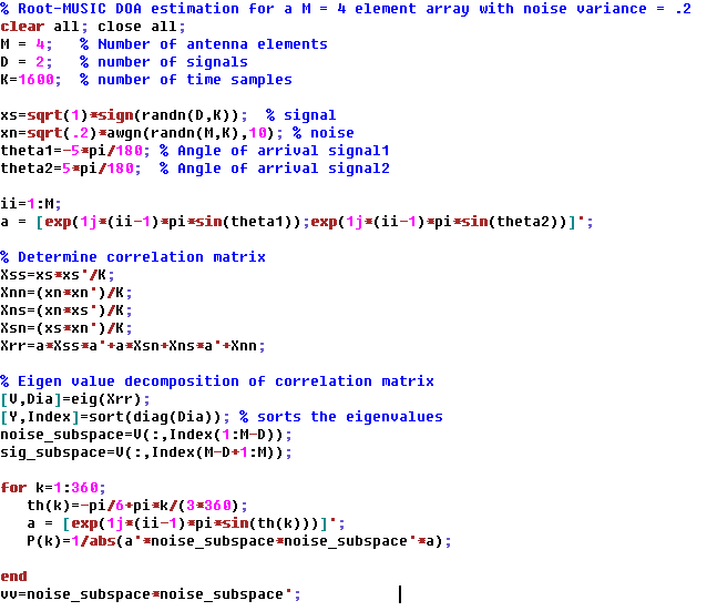
Now let’s focus on the Root-MUSIC algorithm of DOA estimation. The algorithm can be defined as the following steps:

1. Determine the correlation matrix of the arriving signal, noise
2. Determine Eigenvector and Eigenvalues of the correlation matrix. This splits correlation matrix into two subspaces, noise, and signal + noise subspace. Remember that noise subspace corresponds to the maximum eigenvalue.
3. Determine the roots of the pseudo-spectrum polynomial.
4. Determine the roots closest to the unit circle.
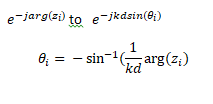
5. Calculate the DOA by comparing to

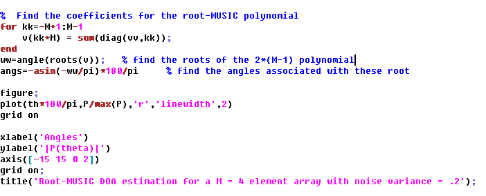
The output of the above script is given below:

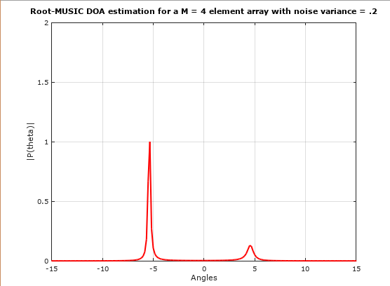
As can be seen from above that by using Root-MUSIC DOA estimation we were able to recover direction of arrival or angle of arrival of both the signals.  (-5 and 5)

The problem of practicality

Although EVD of correlation matrix will give the best performance, we have to take into account computational complexity for implementing EVD. It can be argued that EVD is not efficient to implement on real-time systems even by using most advanced DSPs. Therefore, for practical reasons we need to find another way to achieve this decomposition. In fact, it turns out that Singular value decomposition or SVD are related to EVD, and SVD is more efficient to implement on modern DSPs.

It is worth mentioning here that it is not just about computational complexity. The dynamic range of EVD is twice that of an SVD. More the dynamic range of an algorithm more it is a problem while implementing it on a fixed-point DSPs.

Maybe next time, we will see a comparison between SVD and EVD.

Article Submitted By Mr. Dheeraj Sharma